Part 2.

Orbits of a probe near a black hole:

as a trajectory r(t) and as a path r(φ)

By Alexander Gofen (2026)

Abstract

Unlike in Part 1 where we dealt with a photon, here we study the ODEs representing the static path r(φ) and the trajectory r(t) of a probe approaching a (non-spinning) black hole in a frame of the Schwarzschild model. Contrary to a photon, a probe is a negligibly small pointed mass which may have a variable velocity v < c. Being negligibly small, it does not affect the black hole and the gravitational field in the space: just like it happens with a probe in the Newtonian model, say a satellite near Earth.

In the Newtonian model, according the Kepler laws, a probe moves along one of the conic sections.

Under the General Relativity, however, in the vicinity of a black hole, the motion of a probe is more sophisticated, being described by different types of ODEs.

Here too, we explore those ODEs and graph their solutions using the Taylor Center ODE solver.

Preface

Since Kepler and Newton, the problem of a probe moving in the central gravitational field was well understood as a special simplest case of Newtonian ODEs for the two-body problem, when the mass of the probe may be considered zero. Depending on the initial position and velocity of the probe, it runs along one of the conic sections: the circular or elliptic closed orbits, or parabolic or hyperbolic escape orbits.

The Newtonian model explained the circular or elliptic motion of planets with the then acceptable accuracy. However, there existed a problem with Mercury, whose orbit was not quite "elliptic". The approximate ellipse of Mercury had the eccentricity 0.21 (the highest among other planets), and the big axis of its elliptic shape spun approximately 0.56" per year in a slow precession.

In 1859, the French astronomer Urbain Le Verrier reported that this slow precession of Mercury's orbit around the Sun could not be completely explained by Newtonian mechanics and perturbations by the known planets.

And then, in 1916 Albert Einstein published his General Theory of Relativity. One of its consequences was namely the precession of elliptic orbits of planets orbiting the Sun due to the curvature of the space caused by the gravitation of Sun: the closer to Sun, the bigger the effect. For Mercury, the General Relativity predicted 0.43" precession per year, which was then the only experimental confirmation of the theory.

In the Part 1 we considered another effect of the curvature of the space – the light bending in the proximity of big masses. This effect was experimentally confirmed during the 1919 solar eclipse.

The original equations of the General Relativity are a system of sophisticated nonlinear partial differential equations. However, Karl Schwarzschild in 1915 considered a very simplified setting when the space contained only one non-spinning massive body, and either a massless photon having the speed of light c, or a probe with negligible mass and the speed v < c. Schwarzschild figured out that for this special setting the general equation may by simplified into a system of Ordinary Differential Equations (ODEs). In Part 1 we studied those equations for the case of a photon, and here we are to deal with a system of those ODEs for a probe (called also a test body).

As before, while the trajectory r(t) allows to visualize the kinematic of the motion, r(t) does not exist inside the horizon in the time t of a remote inertial frame. And vice versa, while the path r(φ) does not visualize the kinematic, it shows the curve of the motion in its entirety including the area inside the horizon.

Here, unlike the case of a photon, which has no meaningful proper time τ along its worldline, for a probe it's possible to consider both the global Schwarzschild coordinate time t (as measured by a static observer at infinity), and its own local proper time τ. Thus, for a probe we can describe the motion in three complementary ways:

· Spatial path r(φ): using the static Schwarzschild polar coordinates to see only the shape of the orbit in the plane, without kinematics in time;

· Trajectory r(t): using the Schwarzschild coordinate time t to describe the kinematics as seen in the remote inertial frame;

· Trajectory: using the probe's proper time τ to describe the kinematics along its own worldline.

Consequently, there are three different parameterizations of the same worldline leading to three respective ODE formulations. However, we do not yet have a convenient method to visualize the spatial path in the global Schwarzschild coordinates while animating it according to the local proper time τ. Therefore, in what follows we will restrict attention to the descriptions in r(t) and r(φ), as in Part 1.

The Schwarzschild's ODEs to be used

We are going to use two distinct models for a probe in the vicinity of a black hole or another source of strong central gravitational field:

· a static model visualizing the path or a curve r(φ) or u =1/r(φ) of the probe's motion outside and inside of the horizon;

· a kinematic model visualizing the trajectory r(t) of the probe's motion outside of the horizon.

The notation

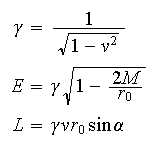
v		The velocity v ∊ [0; 1] normalized so that the speed of light c = 1.
γ		Here v is the length of the vector of initial velocity. Its direction α is encoded into the formula for L.
E		The energy per unit rest mass which is conserved in the kinematic ODEs for r(t) and u(t).
L		The angular momentum per unit rest mass which is conserved in the kinematic ODEs for r(t) and u(t). Here the angle between polar radius r and initial velocity v is α.
G		The normalized acceleration of gravity G = 1
h	h = r₀v₀	The Newtonian conserved angular momentum

Similarly to the case of a photon, for each of the models, we have available ODEs either of the first order, or of the second order.

For u(φ) the first order ODE is

(1)

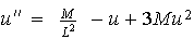
For u(φ) the second order ODE is

(2)

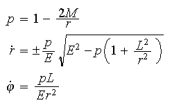
For r(t) the first order ODEs are

(3)

For r(t) the second order ODEs are

(4)

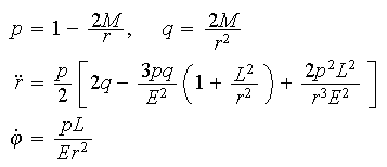
Similarly to such ODEs in Part 1, the first order ODEs (1) and (3) have a square root in the right-hand side with a singularity when the under-the-root content turns into zero. At that, the respective solutions are holomorphic functions even at the points where the square root is zero (for the same reasons as in Part 1). Yet the Taylor integration of a square root at zero is impossible because of the singularity, and such points where v⊥r and r' = 0 inevitably emerge in closed orbits.

The polar ODEs (1), (2) for a probe here look very similar to the respective ODEs (5), (6) for a photon in Part 1. The only difference between the ODE (2) here and (6) there is the term GM/L² depicting the gravitational force acting on a probe, but not on a photon. That is why some orbits of the probe differ from those of photon in the same situation.

We are to use regular ODEs (2) and (4) for integration, while for obtaining the initial values for u' and r' we will sometimes use formulas (1) and (3).

In the kinematic ODEs (3), (4), the physical nature imposes restrictions on the following values: |v| < 1 and r >2M so that E and L be real numbers.

However, for the ODEs (1), (2) in polar coordinate depicting merely the shape of the path, these restrictions may be ignored. In the polar coordinates it's even possible that r < 2M so that the curves extend also inside the horizon, though the derivatives u'(φ) and u"(φ), as well as L² < 0 then have no physical meaning (see the simulation \u(fi)\Circular\InsideM3.scr ).

Properties of ODEs (1)-(4)

All the Remarks 1-5, Theorem 1, and Corollaries 1-2 of Part 1 for a photon hold also for the ODEs (1)-(4) with the only distinction, that for a probe there are infinitely many circular orbits (unlike for a photon). The statements concerning circular orbits in Part 1 apply to any of the circular orbits of a probe.

Circular velocity v_circ

The so-called circular velocity v_circ(r₀) of a probe for a given radius r₀ is particularly important for further study. It's easier to obtain the value v_circ(r₀) from the ODEs (1), (2) as a requirement that

u' = 0

u" = 0

The first one leads to the condition that sin α = 1, meaning that in a circular orbit the polar radius must be perpendicular to the tangent.

The second one translates into the formula:

v²_circ =	M	< 1
v²_circ =	r₀ – 2M	< 1

implying that
	r₀ > 3M
	sin α = 1	.

Consequently, a physically meaningful circular orbit exists for any r₀ > 3M (3M being the radius of the photon orbit) – see simulations in the folder Scripts\u(fi)\Circular\.

Here is a comparative table for the circular orbit and the circular velocity

Newtonian model

Einsteinian model

A probe

A photon

With an assumption that the central body is a point, the circular orbit exists for any radius r₀ > 0. The tangential velocity v_circ(r₀) varies according to the formula v²_circ = M/r₀. At that, when radius r₀ → 0, the v_circ → ∞ which is admittable in the Newtonian model.

For the tangential velocities v > v_circ, bounded orbits still exist and are ellipses. For greater values v > v_circ, the orbits are unbounded, being parabolas or hyperbolas.

If the tangential velocity v(r₀) < v_circ, the orbit is always an ellipse.

The circular orbit exists only for radii r₀ > 3M. The tangential velocity v_circ(r₀) varies according to the formula v²_circ = M/(r₀– 2M). At that, when radius r₀ → 3M, the v_circ → 1 (the speed of light).

v(r₀) > v_circ. For certain tangential velocities v > v_circ bounded orbits exist, though not elliptic. For greater values v > v_circ, the orbits are unbounded, similar, but not identical to parabolas or hyperbolas.

v(r₀) < v_circ. Then the orbit looks like…

· Either a precessing ellipse whose big axis rotates,

· Or a spiral converging to an asymptotic circle of radius r₁, r₀ > r₁ > 3M.

· Or as a so-called zoom-whirl orbit (discussed below), making several tight laps around the asymptotic circle before zooming out into a wide precessing ellipse.

· Or the probe is captured into the black hole

Therefore, in this case, besides the circular orbit at any given r₀ >3M, here exists also an asymptotic circular orbit of radius r₁, r₀ > r₁ > 3M.

In order to whirl into the asymptotic circular orbit of radius r₁, a probe coming from afar must have at its initial position r₀ > r₁ a right combination of its initial velocity v and angle α, discussed in the end.

The circular orbit exists only for radius r₀= 3M. The v_circ(r₀) = c, the only possible speed for a photon: the speed of light.

As no other velocities are possible, the photon orbit r₀= 3M is the only circular orbit. If a photon whirls into an asymptotic spiral, the spiral converges to this only photon orbit.

Unlike for a probe, the type of a photon orbit depends only on its initial position and direction encoded in the parameter b. This parameter has the critical value b = b_crit = 3M√3.

Here are orbits for a photon camming from afar.

b > b_critThe orbits are unbounded, similar, but not identical to parabolas or hyperbolas.

b < b_critThe orbits are captured into the black hole.

b = b_critThe orbit whirls into an asymptotic spiral converging to the photon circle of radius 3M.

Escape velocity v_esc and direction

It's remarkable that both in the Newtonian and General Relativity theories the escape velocity of a probe is expressed by the same formula

At that…

Newtonian model

Einsteinian model

A probe

A photon

With an assumption that the central body is a point, the escape orbit exists for any radius r₀ > 0 and for any angle α ≠ 0 (for α = 0 a probe may collide with the central body).

If v_esc is directed inward, first, the velocity increases being unbounded, and possibly exceeding the speed of light, which is admittable in the Newtonian model.

Later during the escape, it decreases (in accordance with conservation of the full energy: kinetic plus potential).

The escape orbit and escape velocity exist for any radius r₀ > 2M, though not for all directions α for the given r₀ > 2M.

The velocity v_esc cannot exceed the speed of light.

For inward motion at particular values of r₀ and v_esc, the probe will be captured not only for α = 0, but in a certain cone depending on r₀ and v_esc.

For outward motion at particular values of r₀ and v_esc, the probe can escape only within certain cone depending on r₀ and v_esc._.

There is no particular escape velocity because a photon already has the maximal velocity – the speed of light c.

Therefore, the escape orbit depends only on the position of the emitter (r₀ > 2M) and its direction.

Here too specials cones of directions (defined by b_crit= 3M√3) exist in which the photon will be captured into the horizon when b_crit < 0.

At that, for b = b_crit, a photon will be captured spiraling into the photon orbit 3M (rather than into the horizon).

Here are a few examples.

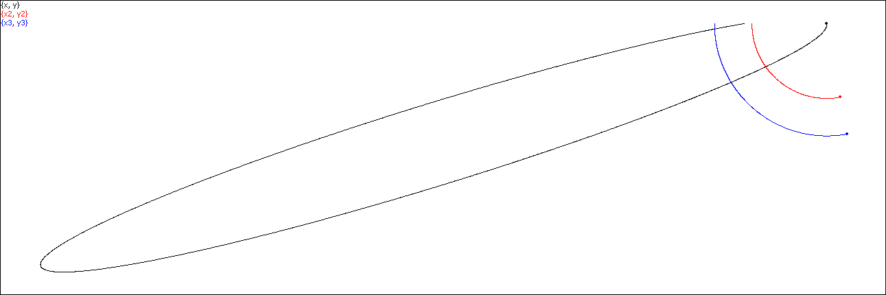
Fig. 1. Here a probe starts near the horizon with a velocity 0.9 outward. It succeeds to move away quite afar.

If it were a photon, it would surely escape. However, unlike a photon, a probe experiences the gravitational pull,

which turns it back to a fall into the black hole. At that, if this probe had the velocity 0.99, it would escape too.

See this simulation in script file \r(t)\FailedEscape1.scr

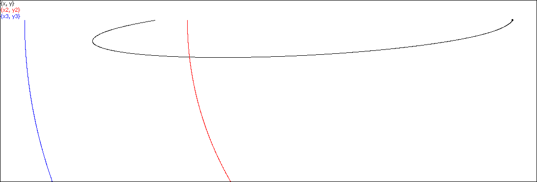
Fig. 2. Here a probe also starts near the horizon, yet with a velocity only 0.6 outward. With this velocity it did not even reach the photon orbit, and then it was quickly sucked into the black hole.

See this simulation in script file \r(t)\FailedEscape2.scr

A Special setting with the initial velocity v⊥r₀

In order of a comparison with the Newtonian model, it makes sense to begin with a setting, in which the initial direction of velocity v is fixed perpendicular to the abscissa and polar radius r₀ so that we vary only the value |v | < c and the distance r₀ from the origin. We will see, that this special situation with v⊥r₀ is possible only outside of the photon circle where r₀ > 3M.

After that, we will consider also the cases where the condition v⊥r₀ does not take place, and possibly r₀ < 3M.

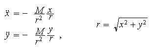
The Newtonian ODEs

(5)

Trajectory x(t), y(t)

in Cartesian coordinates

(6)

Trajectory r(t)

in Polar coordinates

(7)

The path u(φ)

in Polar coordinates

(8)

For comparison, the path u(φ) as in Schwarzschild model

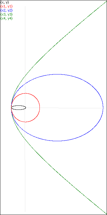
Here, for the initial radius r₀ at φ = π we set the initial velocity v₀⊥r₀. This makes sense because unlike for a photon, a probe has a small mass and may have arbitrary velocity v < c (in our convention, v < 1). Consequently, we can fix the direction of the initial velocity v₀⊥r₀ to vary only its value – and still have an opportunity to study all possible types of orbit behaviors in comparison with the same setting in the Newtonian model.

The picture above demonstrates all the types of orbits with the setting v₀⊥r₀ for the Newtonian ODEs.

Here, we pay special attention to the circular velocity v_circproducing the circular orbit (in red). In this setting only the magnitude of the initial velocity v₀determines which kind of conic the orbit is.

· If we choose v₀ < v_circ , we obtain an inner ellipse (in black), whose right focus is in the origin.

· If we choose v₀ > v_circ (but less than the parabolic speed), we obtain an outer ellipse (in blue), whose left focus is in the origin.

· Otherwise, it is a parabola or hyperbola (in green).

(For every given radius r₀, the value v_circ may be determined from the requirement that the right-side of (6) be zero).

We will see how this Newtonian behavior changes in the Schwarzschild model.

Which type of Newtonian orbits dramatically changes in the Einsteinian setting

The shape of escape orbits of a probe in the General Relativity is similar to the hyperbolic orbits in the Newtonian setting, though they differ from the hyperbolas, as it was demonstrated at the end of Part 1.

However, the bounded orbits of a probe in the General Relativity dramatically differ from the elliptic orbits of the Newtonian ODEs. The Einsteinian bounded orbits of a probe are…

1. Either a capture when a probe gets captured into the black hole.

2. Or precessing ellipsis (unlike steady ellipses in the Newtonian model),

3. Or the so-called Zoom-whirl orbits with precession,

Case (1) of capturing may take place also for a photon, but cases (2) and (3) are unique only to a probe, and we will study them at length in the next section.

Below are illustrations of these three cases.

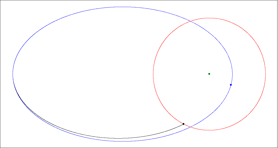
The illustration of case (1) presents a comparison of the Newtonian vs. Einsteinian motion of a probe: as a still image and a movie. The movie demonstrates fundamental difference in behaviors of the Newtonian and Einsteinian motions. The Einsteinian probe (unlike the Newtonian) is…

· Captured into the horizon,

· Slows down near the horizon (from the viewpoint of a remote inertial observer),

· Makes a precession.

Fig. 3. Comparison between a Newtonian probe (in blue) and the Einsteinian one (in black). A small green disk represents the black hole, while the red circumference is the horizon. Click here or on the picture to view the motion as a movie or load the script r(t)\Comparison\WhoFaster.scr

(In the movie, the red disk running along the horizon is merely a software artefact outlining the horizon).

Both probes start at the same position with the same initial velocity (~0.1 c) directed down.

The Newtonian probe moves along the blue ellipse whose right focus is in the black hole. This probe accelerates and decelerates according to the Kepler's laws, and its velocity near the focus is unlimited.

The relativistic probe at the beginning moves almost like the Newtonian. Then, it visibly lags behind more and more until abruptly breaking near the horizon into a full stop. That's how it is perceived at infinitely remoted inertial frame.

In the local frame, however, the relativistic probe accelerates and crosses the horizon inward, its velocity increases approaching (but not exceeding) the speed of light, till it is captured into the black hole.

Another peculiarity of the relativistic probe is that its trajectory represents a precession of ellipse whose big axis slowly rotates.

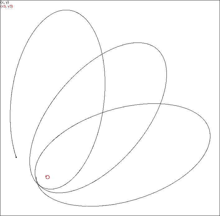
Fig. 4. The simple precession: r(t)\SimplePrecession1.scr

The probe (in black) runs along precessing ellipses where a small red circle is the horizon.

The orbit of Mercury makes similar precession, though negligibly small (just about 1" a year).

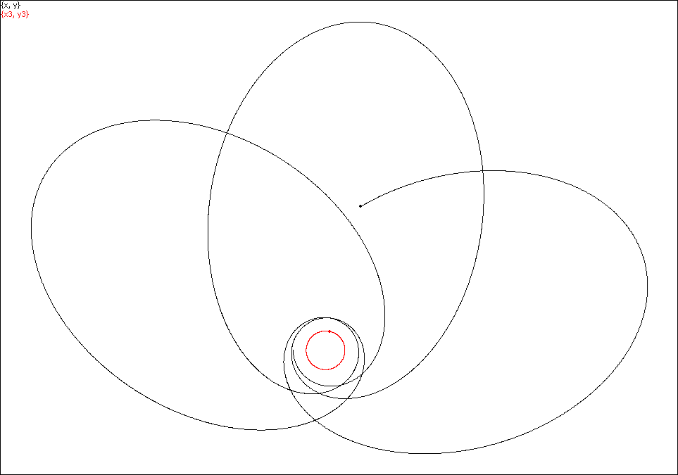
Fig. 5. Unlike the simple precession, here is the precession with the so-called Zoom-Whirl of a probe,

when it makes several tight laps around the photon orbit

before swinging back into a large precessing ellipse again.

A photon can also make a Zoom-Whirl, but it always escapes into infinity if not captured into the photon orbit

because there is no gravitational force acting on a photon which pulls it back.

Computing zoom-whirls

As we learned in Part 1, a photon has the single circular orbit at r = 3M and it may be captured into the photon orbit if its parameter b=b_crit = 3M√3. When this is the case, the path of a photon is a tight spiral asymptotically approaching the photon orbit never reaching and never crossing it (because the under-the-root expression in the ODEs (1), (3) approaches zero never reaching it). In a numerical implementation, however, after several laps along the photon circle, the trajectory of the photon gets either sucked into the black hole, or escapes into infinity (as a consequence of a catastrophic subtraction error in the under-the-root expression). In order to have an escape for sure after several laps, we just need to set parameter b slightly bigger than b_crit – and that would produce something like a zoom-whirl by a photon, though the photon would escape back into infinity after escaping the circle making only whirl without a zoom. This scenario will help us to determine the launch parameters of a probe leading to a real zoom-whirl.

Unlike for a photon, for a probe there exist infinitely many circular orbits for any radius r₁ > 3M. In order that a probe moving from afar be captured into a spiral around the circular orbit r₁, r₀ > r₁ > 3M, the initial velocity of the probe must meet the special conditions

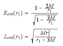
(where the energy E encodes the absolute value of the initial velocity, and L encodes its direction as sin α).

Now let's set a goal, that a probe launched from a position r₀> r₁> 3M be captured into the circular orbit r₁. In order that this happen, the launch parameters of the probe must satisfy the conditions above, which translate into the following formulas for the initial parameters of the probe:

(9)

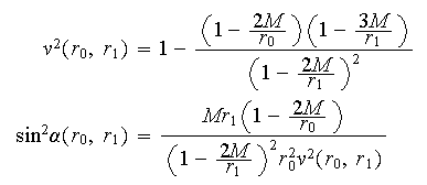
These are the launch parameters for a probe at the initial point r₀so that the asymptotic circular orbit for it be at r₁ and that the probe whirl into an asymptotic spiral around this circular orbit at r₁ : r₀ > r₁ > 3M.

However, not for any pair (r₀, r₁) these formulas above yield the values v²(r₀, r₁), sin² α (r₀, r₁) ∊ (0; 1). It takes some research to obtain an acceptable pair (r₀, r₁).

Let's choose a fixed value r₀ > 3M. Then consider the right sides as functions v²(r₁) and sin² α (r₁), using TCenter for plotting their graphs, which would look like the picture below.

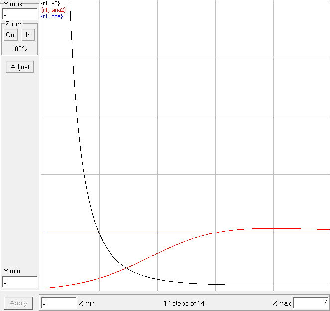
Fig. 6. This is a graph for the functions v²(r₁) (black) and sin² α (r₁) (red) for r₀=10.

You may explore this and other similar graphs via scripts with names workshopN.scr in the folder \u(fi)\ComputedWhirl\.

When the mouse moves on the plotting area, you can see the coordinates of every point.

From this particular graph, we see that the functions v²(r₁) < 1 and sin² α (r₁) < 1 only for r₁∊ (3; 5) – and that's how we can choose a value for r₁ for the formulas above so that every pair (r₀, r₁) would meet the required restrictions, producing an asymptotic spiral around the circle at r₁ which captures the probe – providing that the numerical integration were infinitely accurate (but it is not).

See below in the section " Zoom-whirls for a tangential launch" for the full explanation of which pairs (r₀, r₁) deliver the asymptotic circle at r₁.

Due to the (catastrophic) subtraction error, at close approach to the circular orbit, the trajectory of the probe will finally escape from the circle either outward or inward in unpredictable manner. The values v²(r₁) and sin² α (r₁) produced by the formulas, would provide the maximal number of laps around the circular orbit r₁ which is schievable with this method of integration and 63-bit mantissa.

As our goal here is obtaining zoom-whirl orbits, we must ensure that the escape is surely directed outward. With that in mind, we have to slightly increase the obtained value of sin² α (r₁) by something like 10^-10.

We must modify the value of sin² α (r₁) rather than v²(r₁) because the latter is present in the right-hand side of sin² α (r₁). Therefore, if we modified v²(r₁), that would change also sin² α (r₁) with an unpredictable effect.

Below is one of a zoom-whirl simulations obtained by this method.

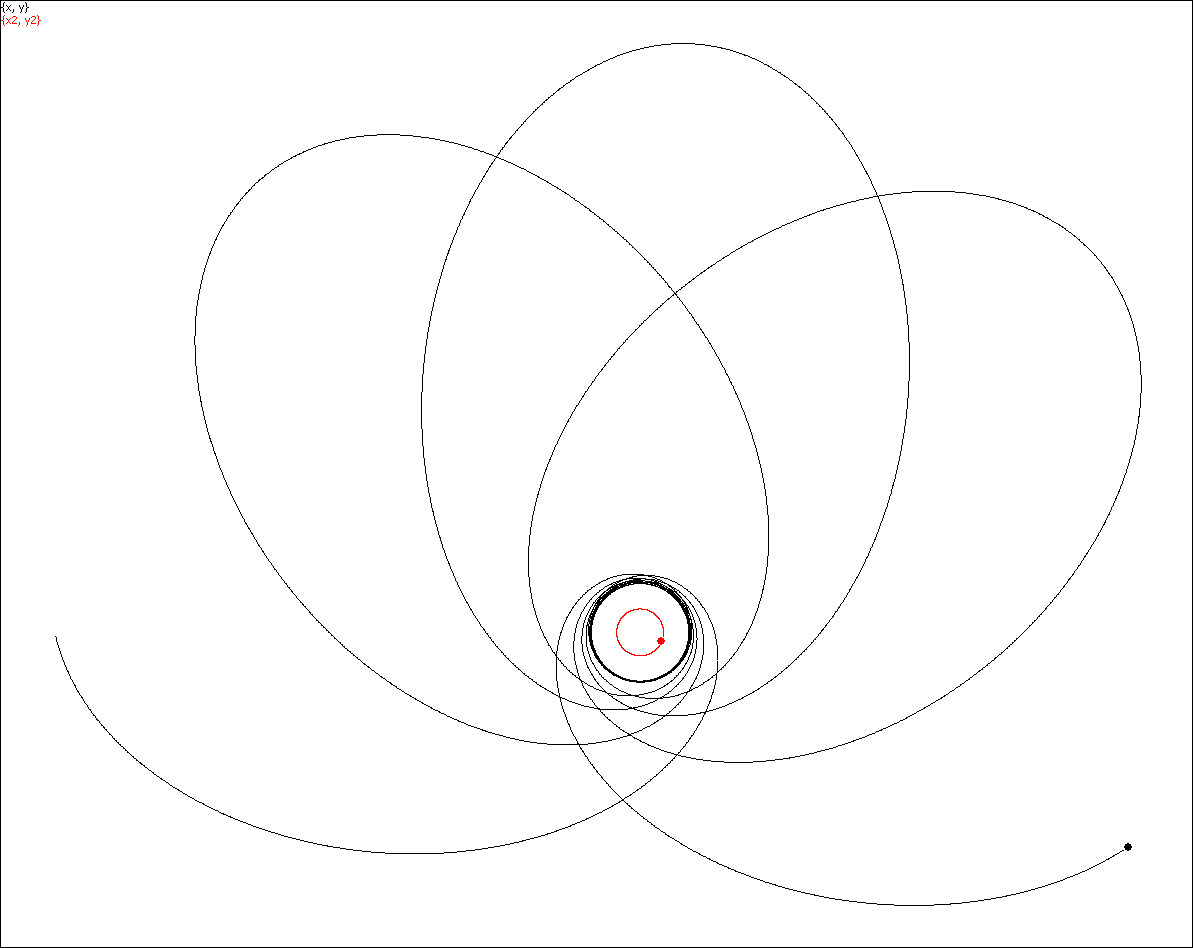
Fig. 7. Here r₀ = 50, r₀ = 4.165, and a probe makes 6 laps around the circular orbit.

In order to see the kinematic animation of this motion in TCenter, load script \r(t)\ZoomWhirl\ZoomWhirl6.scr.

To watch this motion as a movie, click here or on the picture.

Zoom-whirls for a tangential launch v⊥r₀

For any given radius r₀, the formulas (9) provide the launch parameters for entering into the asymptotic spiral as a pair of initial velocity v and direction α of a probe.

However, we are interested in comparison between the Newtonian and Einsteinian models in the specific tangential setting as on the picture at the left in formulas (8). With that in mind, we need to fix sin α = 1 in formulas (9) so that the second equation allows to extract v² and equate it to the v² in the first equation.

In so doing, the system of two equations (9) transforms into one nonlinear rational equation with one unknow r₁. This rational equation may be transformed further into a cubic equation in r₁:

P(r₁) = (r₀ – 2M)Mr₁³ – 2Mr₀²r₁² + (r₀ + 6M)Mr₀²r₁ – 4M²r₀³

We know that one of its solutions must be r₁ = r₀ (the circular orbit at r₀) so that r₁ – r₀ must divide P. It may be verified, however, that r₁ = r₀ is a double root so that also (r₁ – r₀)² divides P. As a result, we solve a linear equation for obtaining first formula (10) for r₁ and then formula (11) for the initial tangential velocity v at r₀.

r₁ =	4Mr₀	(10)
	r₀ – 2M
v =	4M	(11)
	r₀ + 2M

These formulas are remarkable for their simplicity and beauty. Formulas (10, 11) specify the curve {r₀, r₁} of the initial values (r₀, v) for which the tangential path from r₀ falls into the specified asymptotic spiral, i.e. for this path, sin² α (r₀, r₁) = 1. However, there may exist other paths from r₀ falling into the same asymptotic spiral for which sin² α (r₀, r₁) < 1: they are given by formulas (9). The graph below shows the area of points (r₀, r₁) for which the values v²(r₀, r₁) and sin² α (r₀, r₁) produced by (9) meet the required restrictions.

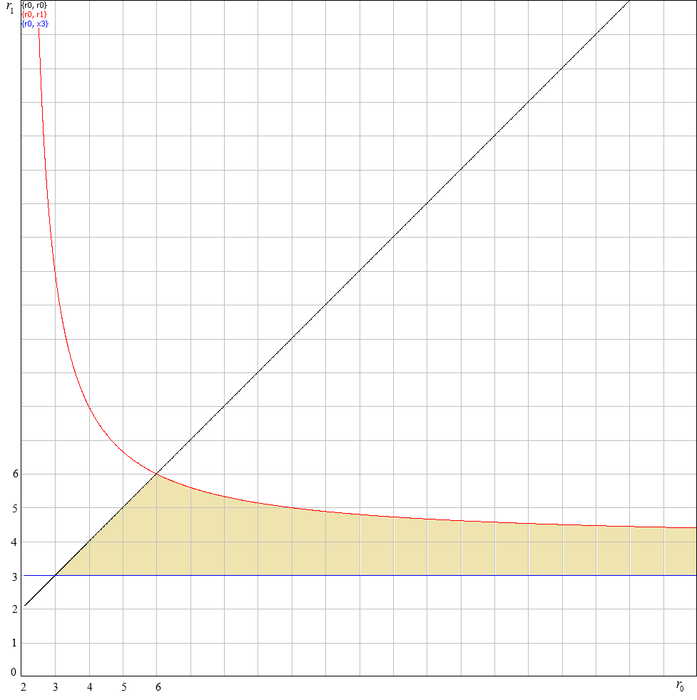
Fig 8. The set (in yellow) of points (r₀, r₁) for which formulas (9) produce the initial values meeting the restrictions.

In this graph M = 1. The red curve is the graph of formula (10): hyperbola with the asymptote at r₁ = 4.

The black line separates the set r₀ > r₁. This script r0-r1.scr is in the folder \u(fi)\ComputedWhirl\.

We see that for the tangential paths we must choose points (r₀, r₁) only on the red curve so that r₀∈ (6M; ∞), and the asymptote is at 4M. For non-tangential paths, we must choose points (r₀, r₁) only in the yellow area so that r₀∈ (3M; ∞), r₁∈ (3M; 6M) and formula (9) for sin α (r₀, r₁) produce the value |sin α (r₀, r₁)| ≤ 1.

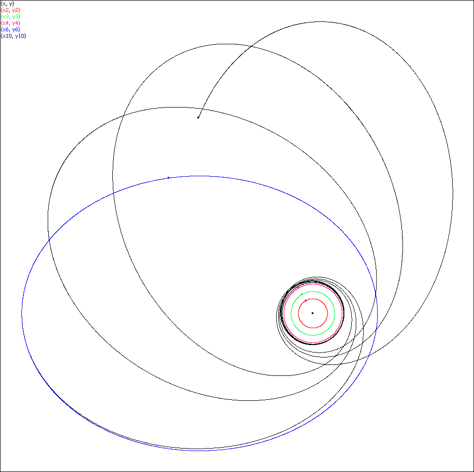
Fig 9. This is a zoom-whirl orbit (in black), the horizon 2M in red, the photon circle 3M in green, and a 4M circle in magenta.

For comparison with the Newtonian orbit (in blue), the initial velocity is tangential. Both orbits have the same initial values at a distance r₀ = 30M > 6M. Consequently, r₁ > 4M.

In the beginning, while afar from the center, the Newtonian and Einsteinian probes move in sync one overlapping the other. The closer to the center, the more their trajectories differ so that the Einsteinian probe enters into the whirl, while the Newtonian keeps running along an ellipse as it should. This script ZoomWhirl40Comparison.scr is in the folder \r(t)\ZoomWhirl\Tangent\ . Click here to view this as a movie, or click over the picture.

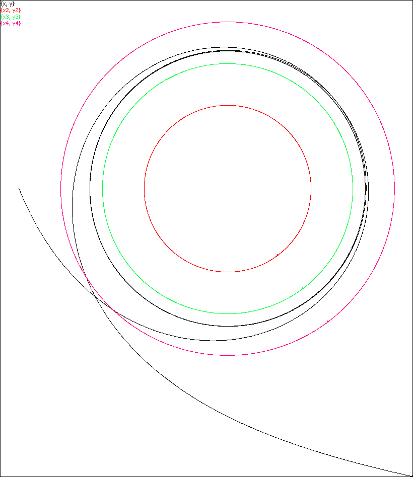
Fig 8. This is a zoom-whirl orbit (in black), the horizon 2M in red, the photon circle 3M in green,

and a 4M circle in magenta. Here the initial velocity is not tangential.

The initial position r₀ = 5M, consequently, r₁ < 4M.

This script ZoomWhirl5-3Esc.scr is in the folder \r(t)\ZoomWhirl\

Using the script file simulations

In order to run all the graphs here as simulations, you have to download and install the TCenter for Windows, following the framed instructions here in the beginning, and then download and unzip the script files of all the simulations in order to navigate to them and load into TCenter.

In simulation of the trajectories r(t), the bullet standing for the probe, moves with the velocity proportional to the velocity of the probe (as perceived in a remote inertial lab).

However, in simulations of r(φ), a visible velocity of the bullet has no physical meaning.

After unzipping, all script files are in the folder ProbeBlackHoleScripts, containing two subfolders (with subfolders):

r(t) – the simulations animating trajectories r(t), demonstrating the kinematic of the motion;

u(fi) – the simulations plotting graphs r(φ).

Inside these folders, there are files and subfolders with self-evident names containing the script files mentioned (and not mentioned) in the article above. For example, the folder \r(t)\Comparison contains scripts in which both Einsteinian and Newtonian motions are presented for comparison in the same simulations.

Among the Auxiliary variables in the scripts of the folder r(t), there is a variable Check standing for the square of the full energy of the probe. You may wish to specify plotting of the curve {t, Check} demonstrating how accurately the energy is conserved in the integration process.

It's worth noting that for circular orbits and for the orbits with the tangential initial velocity it makes sense to specify r'(0) and u'(0) in the pane Initial values explicitly as zeros rather than by the respective formulas (1) and (3). For the tangential setting, these formulas may produce values very close to zero (or even negative) rather than zero. For all other cases when sin α < 1, formulas (1) and (3) are required in the initial values pane.

Finally, here are several illustrations of the behavior of the curves inside the horizon obtained via the ODE for u"(φ) displaying only the shape of the curves and no kinematics.

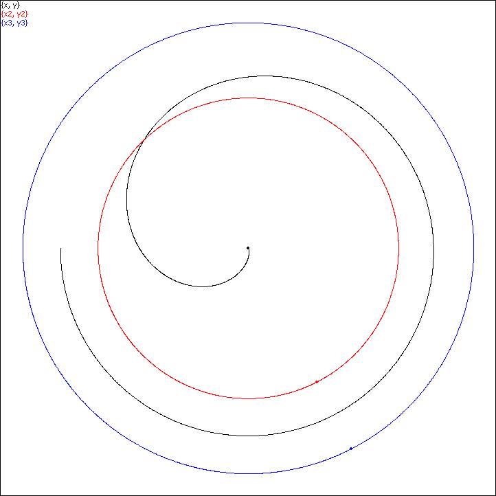
A probe starts at a point between the photon orbit and the horizon and is captured.

Script file InsideM3.scr in folder u(fi)

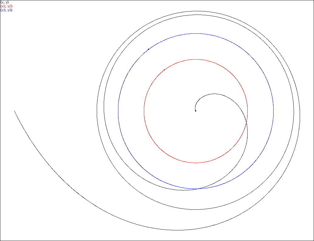
A probe starts at a point outside of the photon orbit and then it is captured.

Script file InsideM2.scr in folder u(fi)

All types of probe orbits near a black hole have been extensively studied and categorized, for example in [1].

References

1. Janna Levin and Gabe Perez-Giz, "A Periodic Table for Black Hole Orbits" (2008), http://arxiv.org/abs/0802.0459v1 and also here.