Lambert W function

https://en.wikipedia.org/wiki/Lambert_W_function

Download this file containing the simulations used here, and unzip it into a folder of your choice. In order to load these simulations in TCenter, navigate to this folder.

This important classical function is fully covered in Wikipedia (the link above). Here we are to explain how to graph and use it in the Taylor Center software TCenter.

The complex function W(z) is defined via an implicit equation

z = We^W.

Its real version is

x = We^W.

The real version of the function W(x) has two branches: the increasing (black) and decreasing (red)  

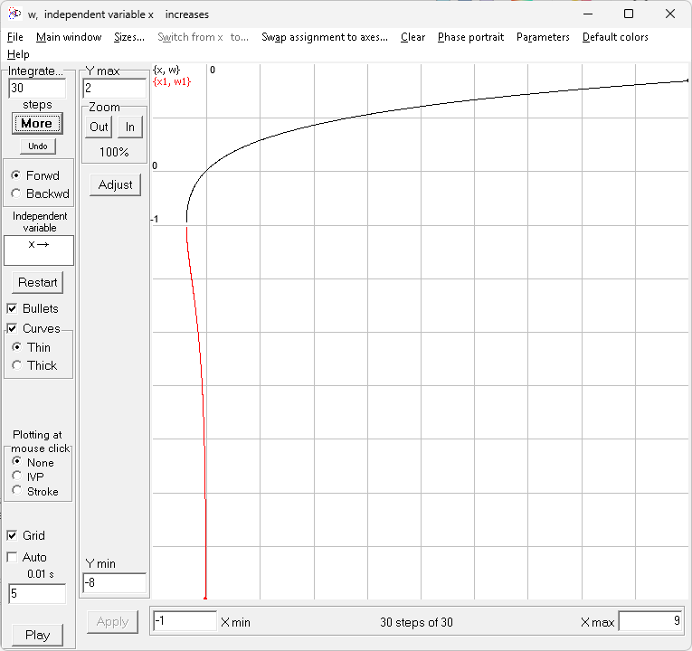
neither of which can be expressed in traditional elementary functions. However, we can differentiate the equation  x = We^W

x' = 1 = W'e^W + W W'e^W = W'e^W (W + 1) + = W' (e^W + x)

so that

W' =	1
	e^W + x

or

W' =	1
	e^W(W + 1)

Observe that the points (x=0, W=0) and (x= –1/e, W= –1) belong to the W(x).

The denominator of  W' disappears at the point (–1/e, –1), and this point of  W(x) is a point of a branching singularity with the monotonously increasing branch W₀ > –1, and the monotonously decreasing branch W₁ <– 1.  

Theorem: In the decreasing branch W₁

             lim W₁ = –∞

x → 0

so that x= 0 is a singularity of  W₁ of the polar type.

Proof. Observe that  W₁(–1/e)  = –1 and  W₁  monotonously decreases so that |W₁| ≥ 1 and increases. As x = We^W and  |W₁| ≥ 1, x can approach 0 only if  W→ –∞. ■

Consequently, the real Lambert function W has two points of singularities: the branching singularity at the point (x = –1/e, W = –1), and the polar singularity in the decreasing branch W₁  at the point x = 0.  

In order to integrate either of the two branches, we must use the initial points on the curve W(x) slightly shifted from the singular point: for the black branch it is the point W₀ = –1+ε, x₀ = W₀e^W₀, and for the red branch it is the point W₁ = –1– ε ,  x₁= W₁e^W1.  Let's set  ε = 0.05.

TCenter allows to integrate either of the branches separately without problems: to integrate either

w = -0.95 x = w*exp(w)

w' = 1/(exp(w) + x) x' = 1

or

w = -1.05 x = w*exp(w)

w' = 1/(exp(w) + x) x' = 1

However, what if we try to integrate both branches

w = -0.95 x = w*exp(w) w1 = -1.05 x1 = w1*exp(w1)

w' = 1/(exp(w) + x) x' = 1 w1' = 1/(exp(w1) + x) x1' = 1

together?

Run the script wStopped.scr (and check the box Grid). Observe, that while the red W₁  branch evolved completely, the black W₀  branch hardly reached the point x = 0. Play it again and pay attention how the red bullet of W₁ moves much faster than the black bullet of W₀. The bullet of W₁ moves down quickly toward big (absolute) values of  W₁  approaching the asymptote x=0 closer and closer.  As the result, the integration step (the same for both variables!) steeply approaches zero so that the integration process stops near  x=0.   

In order to overcome this obstacle, we must diminish the velocity of the bullet of W₁ so that it does not approach the asymptote x=0 so quickly. This goal was achieved in the script w.scr. Run it – and watch that now both branches are plotted completely. When you play it, you see that the velocity of  W₁ bullet significantly diminished. This effect was achieved by introducing a coefficient k in the last two equations:

w = -0.95 x = w*exp(w) w1 = -1.05 x1 = w1*exp(w1)

w' = 1/(exp(w) + x) x' = 1 w1' = k/(exp(w1) + x) x1' = k

Unlike the previous simulation where it was presumed that k=1, now we set k=0.01 so that the velocity of bullet W₁ became 100 times slower. And that was the trick which made it possible to overcome the obstacle.

It's worth noting, that if our goal is only to display both real branches of the function W  without computing it, we can merely specify the inverse function  x = We^W in the axuliary variables and plot it swapping the axes. Run the simulation Lambert.scr to see how it works.